BRAEDEN KEENA

Independent Technical Consultant

Available for contract work

Operations & Business Leader Self-Taught Software & Systems Builder

I built and sold a 500-acre business, then taught myself engineering.

I build data pipelines that know when they're lying to you — backed by operations leadership, validation rails, and embedded RF systems.

🏛️

Operations & Business Leadership

I’ve led teams in places where the stakes were real — 500 acres of operations, city‑wide programs, and engineering projects that couldn’t fail. My leadership philosophy comes from environments where excuses don’t help and clarity keeps people safe.

Explore Leadership & Business Story →

Software & Systems Engineering

Built & shipped web applications, automated scraping pipelines, and federal classifiers (GAScout, GovScout, FindStorage, nacup.us) plus a WiFi-CSI RF hardware sensor array that hit 99.7% device-ID accuracy — then spent two months proving that number was measuring the room.

Explore Technical Projects →
View from the ridge at Honey Lake Motocross Park: riders sitting on their bikes in the foreground, rows of RVs and trailers parked along the valley floor below, and open high-desert rangeland running out to a mountain range on the horizon.
Honey Lake Motocross Park, Milford CA — the 500 acres.

Case study

Room or Radio?

I built a system that identified WiFi devices by their crystal imperfections at 99.7%. Then I spent two months trying to break it, and eventually succeeded.

13of my own working results, killed by controls I built to kill them — out of 29 hypotheses carried to a verdict

0.2σbetween two different boards, four feet apart
19.6σsame board, two rooms
16tested past what the instrument can resolve
99.7% → 29.7%blind holdout, then across sessions

43.4 GB of raw CSI captures — 97 files across 60 recording sessions.This is the corpus, not a result, and it is stated in bytes and files because those are the two things a command can count exactly. The experimental figures above come from two specific 38-minute windows on adjacent nights, each with all transmitters live and the room unoccupied — the conditions travel with the numbers because the numbers change without them. Corpus size and experimental result answer different questions and should never be merged.

Sampling-clock offset over time

B1B2B3

The number I believed

99.7% blind-holdout accuracy at telling three transmitters apart, measured on a chronological split so the test windows came later in time than the training ones. Three ESP32 beacons, a promiscuous receiver, and a signal chain that pulls sampling-clock error out of raw subcarrier phase.

Every radio is driven by a quartz crystal and no two are cut identically. The resulting frequency offsets are baked into the silicon, which is what makes them interesting — they survive a device changing its MAC address, so they promise an identity a spoofer cannot put on and take off.

The number was real. It was not measuring what it was named after.

The part that took two months

The interesting thing is not that the result fell over. It is how many times it got back up first.

The pattern ran for eight weeks. A number would look good. I would find a reason to doubt it, build a test that could kill it, and run the test. Sometimes the number survived. Usually it didn’t, and the fix produced a new good number — which then went through the same thing.

Thirteen of those tests killed a result I already had working. Six of them:

What I believed What killed it
Reference-beacon subtraction cancels receiver-side drift The correction raised the noise floor — in six of six cells
Longer averaging windows reduce estimator noise 256× more averaging moved the pair that mattered 0.69σ → 0.83σ. A time-shuffle control on the identical frames delivered the textbook factor of 16, so the machinery was fine and the signal wasn’t there
Tighter admission gates clean up the marginal pair 175 configurations swept. 174 left it between 0.66σ and 1.18σ
Looser gates recover the ambient devices being missed All 13 recovered sources failed a gain rule frozen before the sweep, at slope dispersions of 9.6σ to 64.5σ
Blind clustering re-links devices across randomized MACs Multi-MAC cluster count came in below the permutation null in all eight configurations — what a one-dimensional feature colliding by pigeonhole looks like
Fusing two features adds information neither has alone +26 pp, winning 12 of 12, CI excluding zero — reproduced exactly by a random number of the same variance

Each of those was a place to stop. Every one had a working number sitting in front of it, and in every case the comfortable thing and the honest thing pointed in opposite directions. The record contains sixteen more questions marked unresolved rather than answered — including one where the positive control failed, which is written down instead of quietly re-run.

None of it explained the original 99.7%.

Then I drew a floor plan

The three beacons live where they live. One on a side table in an open-plan living space, one on a television in a bedroom, one beside a desktop PC in a third room. The receivers are on the living-room wall.

Every between-device measurement the project had ever produced was taken with the transmitters on non-comparable propagation paths. “Which device is this” and “which room is this” had been the same question since July, and nothing in 43 GB of captures recorded where any hardware was.

It is not a bug and no figure was computed incorrectly. It is a design flaw — a variable that was never varied, and therefore never separated from the variable of interest.

The experiment

Move the transmitters onto one surface, four feet apart, and repeat the measurement.

Two boards that had read 7.9σ apart became 0.2σ apart — measured in the same windows, so no amount of clock drift explains it. Two receivers listening to the same transmitter at the same instant, which had been reporting +0.0120 and −0.0121 — opposite signs — agreed to one part in ten thousand. A crystal cannot have one value for one listener and the negative of it for another.

Those two are the load-bearing results, and both are same-instant. The between-night figure is larger and weaker: one board carried from a bedroom to a kitchen counter moved 19.6σ, against a same-position drift floor of 2.5–4.9σ. Real, and a 4× to 8× margin rather than the 19.6× it looks like.

None of it is the behavior of a crystal.

Why this is the case study

Nothing here transfers to a data pipeline. Nobody hiring an engineer needs someone who can fit a RANSAC line to subcarrier phase.

What transfers is the shape of the work: writing the threshold down before running the test, building the control designed to kill your own result, designing tests that can come back either way, and refusing to publish a number without the condition that produced it.

Twenty-nine hypotheses, thirteen of them mine, sixteen questions left open. That is the deliverable.

What happens next, written down in advance

A seven-night replication starts tonight, pre-registered 28 August 2026 before the first capture. Two predictions are on the record: the co-located pair holds below 1.0σ on at least five of seven nights, and reference correction increases cross-receiver disagreement rather than reducing it. If the pair scatters above 1.0σ on most nights, the room conclusion is in trouble — that is the stated falsifier, and it was written before any data existed to argue with.

Then the project closes. Not because it stopped being interesting, but because every remaining test requires hardware I would have to buy, and buying my way to a different answer is not the experiment. Knowing where the end is has been part of the method the whole way through.

I want to work on systems where correctness matters — pipelines feeding decisions, measurements someone acts on, places where being wrong quietly is expensive. I don’t need domain expertise on day one. I need a problem worth being careful about.

Demo

Separation by condition, in standard deviations of the between-unit population spread

Being different hardware moves the measurement 0.2σ. Being the same board in a different room moves it 19.6σ. The two small bars are same-instant measurements; the large one is between-night and carries a 2.5–4.9σ drift floor.

How it works

Write the hypothesis down before running the test

Experiments exist in two stages. Hypotheses, decision thresholds and controls are written to disk and dated before any analysis runs; results are appended below a banner afterwards. Fifteen of the twenty-nine verdicts carry a bar frozen in advance — one of them timestamped 19:30 UTC before the sweep it governed. It means a result cannot be quietly reshaped to fit what came out.

Build the control that kills your own result

Fusing two features appeared to give a +26 percentage-point improvement, winning 12 of 12 comparisons with a confidence interval excluding zero. Substituting a random number of identical variance reproduced the gain exactly: +0.00 pp, CI [-1.80, +1.71]. The finding was dimensionality, not information. That control existed only because it was built to make my own result fail.

Design tests that can come back either way

Two of the twenty-nine ran backwards and made a finding stronger — a cable-topology confound that failed in the opposite direction to what a cable effect predicts, and a suspected artifact that survived removing the correction accused of causing it. A test that can destroy a result is the only kind whose survival means anything.

Chronological splits, never random

Train on the first 60% of each source's observations in time, test on the last 40%. A random split lets the model interpolate between observations minutes apart and reports a number that means nothing about tomorrow. The chronological version is lower and it is the one that describes reality.

No number without the condition that produced it

The headline accuracy was 99.7% on one receiver and 95.7% once a second receiver's captures of the same sessions joined. Same system, same data. Quoting either without naming the receiver configuration is quoting a number that does not exist.

Results

  • Twenty-nine hypotheses were carried to a verdict; thirteen of them were my own working results. Each was live when its test began — reference-beacon subtraction, longer averaging windows, tighter gates, looser gates, cross-receiver library transfer, blind clustering of MAC-randomising devices, feature fusion. Every one was retired by a threshold or control set up in advance to permit exactly that outcome.
  • Two physically distinct ESP32 boards, placed four feet apart on one surface, are statistically indistinguishable — 0.2σ and 0.7σ on two independent receivers, against a between-unit population spread of 0.00237 rad/subcarrier. The same pair read 7.9σ apart the previous night with one of them in another room. Both boards were measured in the same windows, so clock drift cannot account for it.
  • The same physical board reads +0.0552 rad/subcarrier on a television in a bedroom and +0.0087 on a kitchen counter — a 19.6σ displacement of the quantity being used as its hardware identity, for a crystal that never changed. This one is a between-night comparison, so it inherits drift: an untouched beacon wanders 2.5-4.9σ across a single night by the project's own measurement, which makes the honest margin 4x to 8x rather than 19.6x. Stated that way because a reader who opens the drift document would find it in a minute.
  • Two receivers observing the same transmitter at the same instant disagreed by up to 504x more when the transmitters were separated than when they were co-located. With the beacons apart, the two receivers measured one transmitter at +0.0120 and −0.0121 — opposite signs. Co-located, they agreed to one part in ten thousand. A property of a crystal cannot depend on which receiver is listening.
  • Averaging cannot recover the signal, and a control proves the machinery is fine. Allan deviation falls as τ^-0.47 out to about ten seconds and then rises. Shuffling the same frames in time and re-averaging recovers the ideal 1/√W exactly — 15.7, 19.5 and 17.4 against a predicted 16. In true temporal order the same operation yields 1.10 to 1.70. There is nothing left to average away after the first second.
  • An incidental finding: the instrument detects people well. A human in the room appears as an 8.7x increase in spread on every link simultaneously while the medians barely move — a cleaner presence detector than the amplitude-domain pipeline built for that purpose.

Honest limitations

  • This does not show RF fingerprinting is impossible

    Published successes in the field generally use software-defined radios with far greater bandwidth, transient turn-on analysis and controlled channels. What this shows is that ESP32 CSI at 20 MHz, with phase-slope estimation, in a domestic multipath environment, cannot separate the transmitter from the room. That is a statement about an instrument, not about physics.

  • Thermal drift was not ruled out, and three specific versions of it were

    A power-on warm-up transient, an applied one-hour outdoor-to-indoor step, and outdoor air temperature as the drift driver were each tested against controls and rejected. The general mechanism stays rated plausible-but-not-isolated, and the reason is a hardware boundary rather than an analytical one: no temperature was measured anywhere in the corpus — not outdoor, not indoor, not on-die. Isolating it needs an instrument the project does not own, so the honest position is three named sub-hypotheses rejected and the category left open. Naming the three is a stronger claim than naming the category, and the difference is not cosmetic.

  • One window per condition, and a seven-night replication is running to fix it

    The 0.2σ co-location result is a single 38-minute window. It does not inherit drift — both boards were measured in the same minutes — but n = 1 is n = 1. A seven-night repeat is under way, pre-registered 28 August 2026 before the first capture. Two predictions are on record: the co-located pair holds below 1.0σ on at least five of seven nights, and reference correction increases cross-receiver disagreement rather than reducing it. A third asks whether the 1.0σ bar is even resolvable given a documented 2.5-4.9σ drift floor — because if it is not, the honest verdict is that the design cannot answer the question, which is a different outcome from the prediction failing. The registration separates those two before any data exists to blur them.

  • The receiver-disagreement result was not pre-registered

    It was found by checking a caveat rather than by testing a frozen hypothesis, so no threshold was written for it in advance. The direction and magnitude should be predicted beforehand and re-tested on a fresh capture before it is treated as established. It is reported at the same prominence as the findings that were pre-registered.

  • Power source is confounded with device identity

    In the co-located capture two beacons ran on battery and one on mains. The collapse between the two indistinguishable boards survives this — they differ in power source and collapse anyway, which is the harder direction for a confound to explain. The third board's apparent distinctness does not survive it, and is not relied on.

  • Three devices, and the class count travels with every figure

    Every accuracy number here is against N = 3 with chance at 33.3%, and the count is printed beside each one. An earlier figure in this project became permanently uninterpretable because its class count was never recorded, and that is not being repeated.

  • The dataset is not published, and results cannot be independently re-derived

    Running promiscuously, the array captured every WiFi transmitter in range — including third-party hardware whose owners did not consent — and the captures are unavoidably a log of when a home was occupied. That is a privacy decision before it is a reproducibility one. The pipeline can be read in full; the data behind the numbers is not shipped, and this is stated rather than worked around.

Tech stack

Firmware

C on ESP-IDF v5.5 · ESP-NOW transport · custom binary telemetry protocol · task and RF-liveness watchdogs · NVS-persisted node identity

Signal processing

Python · NumPy · vectorized RANSAC · phase unwrap with temporal continuity · 1D Kalman drift tracking · Welford covariance · Mahalanobis distance with χ² thresholds

Analysis and data

DuckDB · Parquet · SQLite · chronological train/test harnesses · pre-registered experiment scripts · bootstrap resampling · permutation and variance-matched null controls

Deliberately not used

deep learning frameworks — every decision the system makes is explainable as an ellipse and a probability

What's next

Landing soon

  • Digital fingerprint matching at scale

    Maturing the live match/library workflow so any capture is scored against the learned device library in real time, with four operational verdicts: known device, same radio on a rotated MAC, trusted MAC but wrong radio (investigate), or stranger.

Cracking the clock-twin frontier

  • Thermal compensation from the transmitter itself

    Every ESP32 has an internal die-temperature sensor. Embedding TX die temperature in the beacon payload lets the host correlate and compensate the thermal drift that currently smears same-model centroids together — zero added hardware cost, and the single highest-value improvement on the board.

  • Higher-dimensional features

    The current model uses two features (CFO, SFO) and discards the per-subcarrier phase residual shape, which carries multipath and hardware-nonlinearity signature. Adding a residual-vector feature to a higher-dimensional Mahalanobis model is the path past the same-model ceiling — and it can be validated against the existing 2.36M-frame dataset with no new captures required.

Hardware & deployment

  • Custom 3D-printed enclosures

    Turning the breadboard prototype into a finished, mountable sensor product — designed in OpenSCAD, printed in-house. Hardware photos land here as soon as the first enclosure run is off the plate.

  • Raspberry Pi host migration

    The collector is pure Python and pyserial, and runs unchanged on a Pi — enabling a permanent headless deployment with home-automation (MQTT / Home Assistant) publishing, and the eventual live embed for the demo slot above.

Operations leadership

Running the thing, not just building it.

Operations work sits behind the engineering — permits, payroll constraints, safety programs, and the people who have to be somewhere at a specific time for any of it to work. Two of those jobs are written up in full.

Honey Lake Motocross Park

Founder / Sole Operating Partner · Honey Lake Motocross Park, Milford, CA · 2016–2018

A two-day race weekend that peaked at 6,500 attendees, ~1,200 of them racing, directed by a 120-person crew of staff, contractors and volunteers with full P&L responsibility throughout — and no payroll budget for any of them.

~500Acres acquired and returned to operation
1,200Riders at peak weekend
120Staff, contractors and volunteers directed
The rebuilt start straight at Honey Lake: groomed hard-pack dirt running toward the hillside track, with snow-capped mountains behind it.
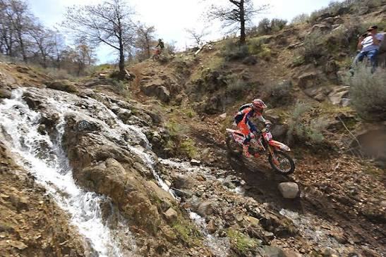
Riders working through the rock section of the Honey Lake track while spectators watch from the bank above.

Read the full Honey Lake Motocross Park case study →


School Crossing Guard Operations

Crossing Guard Operations Supervisor · All City Management Services (ACMS), Blue Valley USD 229, KS · 2023–2025

Ran crossing-guard operations for the southern half of Blue Valley USD 229 — 50 guards across 33 sites, staffed twice a day, which is 66 individual posts to fill every school day. No post went unfilled and no student was injured across the full tenure.

50Crossing guards hired, trained and managed
33Sites covered, staffed morning and afternoon
66Individual posts to fill every school day

Read the full School Crossing Guard Operations case study →

Background

The operations years and the engineering years aren’t as separate as they look on paper. Both come down to the same habit: don’t trust an unverified result, find where the system actually breaks, and be straight about what still doesn’t work.


Operations experience

Technical skills

AI & Agentic SystemsAgentic Engineering & AI Coding Tools (Claude Code, Antigravity/AGY) · Empirical Test Harnesses & AI Verification · LLM API Integration & Automated Workflows

DevOps & AutomationGit / GitHub · CI/CD (Cloudflare Pages, Netlify) · Windows Task Automation · Scheduled Data-Refresh Engines & Validation Rails

Hardware / IoTESP32 Firmware (C / ESP-IDF) · ESP-NOW & BLE Protocols · I2C & SPI Sensor Networks · RF Signal Processing (WiFi-CSI) · 3D Printing & CAD (OpenSCAD)

LanguagesPython (scraping, data pipelines, automation) · JavaScript / TypeScript · SQL · HTML5 / Modern CSS

Operations & LeadershipFull P&L Responsibility · Teams of up to 100 People · Vendor & County Permitting · Emergency Safety & Medevac Planning

Web & DataAstro v5 (Content Collections & SSG) · REST APIs & API Reverse-Engineering · Technical SEO & Schema.org JSON-LD · Leaflet.js & MarkerCluster Mapping · JSON & SQLite Data Architecture

Other work

Selected work.

Multi-Platform Communications ConsolidationClient engagement

Delivered · Jul 2026

The client came to Upwork looking for basic Python scripting for a legal proceeding. What the matter actually needed was a small ETL system: five communication platforms, no shared identifier between them, and a timeline where an hour of timezone error could misstate what happened when. This is what got built instead of a script — a pipeline designed to be checked, not just to run.

7,626records parsed and normalized across five heterogeneous communication sources
5platforms unified into one timeline: Gmail, iPhone SMS, WhatsApp, Facebook Messenger, and webmail
31 Jul 2026delivered on Upwork — client has since engaged him for the next phase
“I originally searched for someone who could handle basic Python scripting, but Braeden delivered far beyond that. He anticipated needs I didn't even know how to articulate.”
Client, Upwork★ 5.0

The client has since engaged him for the next phase of this project.

A client came to Upwork needing help pulling together records for a legal proceeding. What the case actually needed was full-scale data engineering: 7,626 messages and records were scattered across five incompatible export formats — Gmail, iPhone SMS, WhatsApp, Facebook Messenger, and a webmail account — each with its own timestamp convention, its own missing fields, and no shared identifier to link them.

The pipeline parses each source’s native export format, then normalizes every timestamp to a single timezone with correct daylight-saving handling — a naive UTC conversion silently shifts events by an hour on either side of a DST boundary, which is disqualifying when timing is part of the record. Duplicate and fragmentary records are reconciled across sources into one chronological timeline, and every surviving record carries a provenance tag back to its original source file, so any line in the final output can be traced to exactly where it came from.

The deliverable was a formatted PDF report generated automatically from the reconciled dataset, plus a dedicated QA audit pass — a second, independent check of the pipeline’s output against the source exports before delivery — because a consolidation this size is only useful if it’s also correct.

Why it mattersThe client came in looking for basic Python scripting. What the underlying legal proceeding actually needed was full-scale ETL: five incompatible export formats reconciled into a single record with defensible provenance for every line — the kind of problem that doesn't get solved by a script, only by a pipeline built to be checked.

Python · ETL & data reconciliation · Timezone/DST-aware normalization · PDF report generation

GAScout

Live · 2026

Built because Georgia's delinquent-tax data exists only as a 9,915-page fixed-width mainframe PDF — a format built for a printer, not for analysis. The extraction engine's job is to turn that dump into something a policy researcher can query, cut, and trust: parsed and checksum-verified line by line, with zero dropped rows, so aggregate figures are traceable back to source instead of estimated.

$62.75Muncollected delinquent tax liability tracked across 8 tax cycles
409,142line items parsed from 9,915 mainframe PDF pages with 0 dropped rows
90automated offline test fixtures verifying parser & checksum integrity

A static public-records intelligence dashboard and daily extraction pipeline built on DeKalb County delinquent tax listings.

County tax listings are published as a monolithic 9,915-page fixed-width mainframe PDF file (DQ205GADEK). The python extraction engine ingests the document offline line-by-line, detecting and auto-correcting 32 column-overflow shifts via a 5-column checksum verification algorithm. The pipeline enforces 100% line accounting — zero dropped rows, zero malformed records — backed by 90 automated offline test fixtures.

The web interface presents aggregate financial insights without publishing personal PII:

  • Tax Year Trend Explorer: Multi-metric trend analysis showing how 56.9% ($35.7M) of outstanding debt sits in the 2025 cycle, while 26,000+ 2018 records remain open as long-tail “zombie properties”.
  • Pareto Economic Breakdown: Highlighting how 77.8% of rows are micro-bills under $100, whereas just 1,023 bills (> $5,000) hold over $11.3M in debt.
  • Interactive Policy Collection Simulator: Live threshold tool allowing policy researchers to test collection targets ($100, $500, $1,000, $5,000+) to calculate recovered revenue ($M), percentage of county debt cleared, and owner contact efficiency.
  • Georgia Tax Status Classification: Clear breakdown detailing Fi.Fa. Lien Execution (F), School Tax Delinquency (S), Assessment Appeals (A), and Claim Transfers (T).

Why it mattersThe checksum verification isn't a nice-to-have: it's what auto-corrected 32 column-overflow shifts in the source PDF and let the pipeline enforce 100% line accounting — zero dropped or malformed rows. That's what makes the $62.75M liability figure something a policy researcher can trust down to the row, not a rough estimate off a monolithic government PDF.

Python · Astro v5 · Vanilla JavaScript · Cloudflare Pages · pypdf

GovScout

Live · 2026

Built to do what a busy contracts specialist doesn't have time for: read every new SAM.gov solicitation in a given commodity area and flag the ones actually worth a phone call. It scores solicitation copy for pricing-availability signal and extracts the National Stock Numbers and part quantities buried in the text, so a human only has to look at the solicitations the scorer says are worth looking at.

100/100pricing-availability signal scoring algorithm across 4 keyword families
NSN & P/Nautomated regex extraction of National Stock Numbers & part quantities
0 Depszero third-party dependencies beyond standard library & pytest suite

A federal procurement monitoring engine modeled on defense logistics (DLA/DIBBS) RFQ tracking. GovScout ingests live solicitations from the SAM.gov Opportunities API v2, filters them by FSC/PSC codes, detects pricing-availability signals, and extracts structured part data into SQLite.

  • Pricing Signal Classifier: Evaluates solicitation copy against weighted keyword families (online_pricing, historical_pricing, quote_workflow, competitive) to generate a 0–100 pricing feasibility score.
  • Structured Part Extractor: Automatically parses National Stock Numbers (NSN \b\d{4}-\d{2}-\d{3}-\d{4}\b), manufacturer part numbers (P/N), and required item quantities from raw text.
  • Dual Mode Architecture: Operates in Live Mode (REST API client with 0.5s rate-limiting, 429 backoff, and state persistence) and Demo Mode (bundled offline dataset for zero-network testing).
  • SQLite Engine & Report Generator: Upserts normalized solicitations with duplicate detection and exports CSV feeds and console digests grouped by signal priority.

Why it mattersZero third-party dependencies means the pricing-signal classifier, the NSN/part-number extractor, and the SQLite engine are auditable end to end — nothing opaque to trust in a pipeline that's deciding which federal solicitations are worth a human's time.

Python 3.11 · SAM.gov API v2 · SQLite · Regex Signal Classifier · pytest

Health-Inspection Lead Pipeline

Live · Aug 2026

A small business needed to know who to call first. The records that answer that are public, published by county and city health departments, and available in completely different shapes depending on who publishes them. The pipeline itself took a few days. The rest of the time went into the parts that stop a lead list being confidently wrong — a source whose join key is misspelled, a server that returns HTTP 200 for records that don't exist, and one jurisdiction that got investigated in full and then deliberately not built.

1jurisdiction researched in full, then deliberately not built
279tests, none of which touch the network
~30requests to cover a 9,711-business county
2publisher shapes: a JSON API and reverse-engineered HTML

Businesses cited by a health inspector for a broken or dirty ice machine have a dated, documented problem with a specific piece of equipment. Those citations are public record. Turning them into a ranked call list is a day of work. Making sure the list is right took the rest of the time.

Two publishers, two entirely different problems

Santa Clara County publishes on Socrata — a real JSON API, three tables joined client-side, about thirty requests to cover 9,711 businesses.

Washington DC publishes through Tyler’s Digital Health Department platform, which has no API at all. One GET returns one server-rendered inspection report, and all four query parameters are required, including an undocumented tenant id. Inspection ids are sequential integers. None of it is written down anywhere; it was reverse-engineered.

Both feed one deduplicated, scored list, and every lead carries the market it came from.

The join key is misspelled, and correcting it breaks everything silently

Santa Clara’s inspections table names its join key inpsection_id — p and s transposed. The violations table spells the same key correctly. Both are right; they disagree with each other, because Socrata derives field names from the uploaded column header and the typo is baked into the dataset.

Correcting the spelling doesn’t raise an error. It produces an empty lead list, which looks exactly like a quiet week. The constant carries a large comment and is pinned by a test named test_join_key_typo_is_deliberate, so a future tidy-up has to argue with a failing test rather than with nothing.

DC has the same shape of trap from the other direction: requesting an inspection id that was never issued returns HTTP 200 with a normal-looking page. The only usable “this record doesn’t exist” test is a string check on the body.

Florida: researched in full, then not built

Florida’s mechanism was worked out completely — the free bulk extract, the per-district partitioning, the licensure file that joins phone numbers, all thirty-five of its columns enumerated to confirm what it does and does not carry. It carries no email address.

No adapter was written. The finding was that Florida is better served by a public records request than by scraping, and the document explaining why is in the repository next to the adapters that were built. Deciding not to build something is a result, and it is only useful if it is written down where the next person will find it.

Rate limiting, and correcting my own first version

Version one used random.uniform(1.0, 2.0) between requests and described this in its own comments as “human-like delays” with “zero bot-detection footprint.”

That posture is wrong for a documented public API that publishes a crawl delay. The rewrite honours the published Crawl-delay: 1, sends a descriptive User-Agent with a contact address rather than a browser string, honours Retry-After on 429, backs off exponentially on 5xx, and caps the entire run at 400 requests so a bug cannot become a hammering. Both jurisdictions share one budget, so adding a second market did not silently double the traffic.

The correct behaviour on a public API is to identify yourself and stay inside the published limit, not to look like a person.

What the source doesn’t have, reported as its own output

Every run writes a coverage report and a request trace: what was retrieved, what failed, what was deliberately skipped, and which fields the source simply does not populate. An empty result has to distinguish no data exists from the request failed from I never asked — three things that look identical in a lead list and mean completely different things.

Two more that are stated because leaving them out would mislead. Santa Clara’s data carries no explicit open licence — Delaware’s equivalent is marked public domain and San Francisco’s carries PDDL, and Santa Clara’s metadata carries neither. Access is permitted and the records are public, but there is no licence grant to point at. And the dataset goes back exactly two years and no further, because it was created in August 2024 — there are no older records being filtered out, the source does not have any.

Two fields where one would have been easier

jurisdiction is the publisher’s boundary and the deduplication key. market is the sales territory and the label a human reads. Collapsing them into one field would either put a county name on someone’s call list or use a marketing label as a data key.

The first version exported everything as “San Jose.” It is a county dataset covering twenty-three cities.

The daily run refuses to send stale mail

The emailer reads a CSV. It has no way of knowing whether that file was written thirty seconds ago or last Tuesday. On one run the collector found 246 leads and wrote none of them, because the file was open in a spreadsheet and locked — the pipeline reported that correctly, but an emailer running blind straight afterwards would have sent the previous list with the current date on it.

So the wrapper sends only if the file was written by that run, and the digest covers net-new leads only. On a day with nothing new it stays silent, which is the honest output and the one that keeps the mail worth opening.

Why it mattersThe list decides call order and nothing else. The citation that put a business on it is never mentioned to that business, and nothing in the repository generates anything to say to one — a rule written into the README's third paragraph before the first adapter was built.

Python · Socrata SODA API · server-rendered HTML parsing · pytest — 279 tests, no network · per-run request budget with backoff · coverage and trace reporting · PowerShell scheduled task

findstorage

Sunset · 2025–2026

It started as an internal problem: a five-digit store identifier the team I was on needed every day wasn't published anywhere. The tool that found those numbers turned into a national directory, and the pricing data came with it. Built to run unattended and stay correct when the market moved — when an operator merger added roughly 1,100 stores overnight, the daily pipeline absorbed it with zero manual intervention rather than needing to be rebuilt around it. Collection ended 25 August 2026 after I re-read the source's terms of use; the site stands as a dated archive.

48 daysconsecutive daily snapshots, zero gaps, 4,664 stores in 43 states
396,402advertised price changes logged, every figure reproducible from a named script
88.7%of tracked inventory repriced in a single day — the largest of thirteen such events

This began as a store-ID finder. A five-digit site number that the team I was on needed daily wasn’t published anywhere, so I built the thing that found them — and the market data came along for free. It grew into a national directory of advertised self-storage prices and the research that falls out of tracking them over time.

A seven-pass discovery scraper collected publicly published rates for 55,332 advertised price points across 4,664 stores in 43 states, running itself daily through GitHub Actions with commits landing unattended. The pipeline had safety rails: a run aborted rather than publishing if store count dropped below a floor or fell more than 10% against the previous run. It took 48 consecutive daily snapshots with no missed days, and the rate-change log holds 396,402 advertised price changes and 148,870 promotion changes. When a large operator merger added roughly 1,100 stores overnight — a ~30% jump — the pipeline absorbed it cleanly and surfaced the shift in the trend data instead of choking on it.

Collection ended 25 August 2026. Before adding a second operator to the dataset I sat down to read their terms of use, which raised the obvious question of when I had last read the first operator’s. Theirs prohibits automated collection. I stopped the same night, disabled the scheduled job, and the site now stands as a dated archive rather than a live directory. The engineering below is what the project was; none of it depends on the collection continuing.

What 48 days of daily snapshots turned up

Advertised rates do not drift. They sit completely still for days and then move in coordinated waves. On 18 of 46 days not a single tracked rate changed; on thirteen days, tens of thousands did. Nothing observed falls between those two states — the busiest quiet day logged 2,443 changes and the smallest wave logged 12,792.

The largest wave repriced 88.7% of tracked inventory in one day. Individual stores move decisively and in opposite directions within the same wave, at three to five times the rate a shuffled null predicts, so the national median can sit flat while most of the book moves under it.

One 5×5 unit shows the mechanism in seven rows. Its advertised list rate changed eight times in six weeks while the promotional badge on the page never changed. Between 20 and 22 August the advertised saving grew from $123 to $176 — and the first month went from $46 to $66. The discount is a fixed percentage; the number it is a percentage of is not.

The analysis I care most about is a matched-pairs design. Averaging prices confounds the attribute with the market — climate-controlled units are more common in expensive metros, so a naive average credits the feature for the city. Instead it compares units of the same size, at the same store, differing in exactly one attribute (climate control, floor level, drive-up), so location and local demand cancel out and what’s left is closer to the price of the attribute itself. Climate control carries roughly an 18–22% premium on that basis. Records are linked across sources by 150m haversine distance plus ≥60% name-token overlap.

Everything is cut by size (locker through 10x30 and parking). 414 ZIP3 markets are computed nationwide rather than hand-picked, each with a client-side drill-down: store count, units per store, promo share, median price by size with price-per-sqft against the national figure, trend sparklines, and a renter leverage score. Movers tables surface the largest availability drops and restocks and the largest 10x10 price moves over a rolling window, and a per-store price-history view charts a single store’s advertised prices over time by unit size. Moving the detail data into a sidecar fetched on first interaction kept the whole drill-down to +3.6KB gzip on initial load.

How the numbers were checked

Every failure below was found in my own data, by me, and every one of them had been quietly wrong for some length of time before it was caught. They are on the page because the corrections are the part worth reading.

A number with no command behind it decays. A hand-typed coverage figure turned out to be wrong by 5.6×, and had been wrong for an unknown period — nothing in the pipeline could say how long, because nothing had ever recomputed it. Every published figure is now emitted by a committed script on each run, and the script refuses to write its output file if any value comes back null. A stale number never drifts randomly; it drifts in the direction that flatters the page.

Counts and statistics have to describe the same rows. 56 rows in the rate log recorded a price moving from zero — a unit arriving in the dataset, not a repricing. They were excluded from the medians but still counted in the daily totals, so two numbers on the same page were computed over two different populations. The filter now runs before the tally rather than after it.

Derive the window from the thing that defines it. The observation window was originally read off the change log, which meant days with no changes weren’t days at all. It reported 41 days and 13 zero-change days. Taken from the snapshot dates instead — the actual record of when the scraper ran — the real figures were 44 and 16. Three days had vanished because nothing happened on them.

A step in the data is not a movement in the market. Twice the tracked population changed size sharply: 441 stores entered on 9 July and 1,096 on 23 July, the second being a merger. Averages across those dates compare two different populations. The breaks are detected from the store counts rather than asserted from the news, and every chart that crosses one draws it as a labelled rule — because the misreading being prevented is someone glancing at the shape of a line.

Zero is not the same as nothing. 9,164 of 34,416 store-size listings are quarantined from the movers tables, each with a named reason recorded to a CSV. The one that matters most: a store whose advertised availability drops to exactly zero and stays there has stopped publishing availability, not rented out its entire inventory. Ranked naively it would be the largest mover on the page and the least likely to mean what it says. The same logic runs in reverse for stores that begin publishing.

Test the pattern against a null. The claim that individual stores move coherently — decisively, and in opposite directions inside the same wave — is measured against a shuffled null rather than eyeballed off a chart. Stores move together at three to five times the rate the shuffle predicts.

Fail loudly, in the right direction. A run aborts rather than publishes if the store count drops below a floor or falls more than 10% against the previous run, so a source changing its markup surfaces as a stopped pipeline the same day instead of as quietly missing rows. The failure mode that costs you is the one that still produces plausible output.

Worth stating plainly: these are advertised online rates, not what any given renter ends up paying. Coverage is whatever the discovery pass found published, so it is a sample rather than a census, and matched pairs control for store and size — not for everything. The dataset is closed as of 25 August 2026 and will not be extended.

The findstorage directory view: a filter bar and a grid of store cards, each listing site number, address, phone, and a per-size table of advertised monthly prices and promotions.
Directory view — advertised price by unit size for each store, including stores with no vacancy.
The findstorage trends page: national advertised inventory and national median 10x10 price plotted across daily snapshots from April to July 2026.
Trends — national advertised inventory and median 10x10 price across daily snapshots.

Why it mattersIn late July 2026, a National Storage Affiliates merger added roughly 1,100 stores to the market overnight. The daily discovery pipeline absorbed it with zero manual intervention: stores tracked jumped ~3,539 → 4,637, advertised inventory rose ~212,000 → ~292,000 units, and computed ZIP3 markets grew 354 → 414. The safety rails held, and the merger showed up as signal in the trend data instead of a system that needed babysitting.

Python · Vanilla JavaScript · Leaflet.js · GitHub Actions · Cloudflare Pages

nacup.us

Live · 2026

Built because World Cup 2026 news and local watch-party info lived in a dozen different places and nowhere at once. It's a single aggregation-and-generation pipeline: news from 16+ feeds deduplicated and ranked by relevance, venues merged from four independent sources into confidence-scored records, and the whole site rebuilt daily so every team, match, and city page stays current without anyone touching it by hand.

48 hrsconcept to deployed production site
700+visitors on day one, first-page organic search within 24 hrs
80+programmatically generated SEO pages across 38 host cities

Built because I wanted one place for everything World Cup 2026 — every morsel of news, plus which bars and fan events were happening near me. It became my own daily driver during the tournament, and drew around 1,500 unique visitors a month while the World Cup was on.

News is aggregated from 16+ feeds and ranked by a time-decay scoring formula that weighs source credibility, team and player entity matches, and whether a team is playing that day — with near-duplicate coverage clustered instead of repeated. The venue map merges Yelp, Foursquare, OpenStreetMap and Google Places into single records using geographic proximity and name-token similarity, each carrying a confidence score based on how many independent sources agree.

A daily GitHub Actions pipeline regenerates the site — 48 team pages, 99 match pages, 38 city pages and a 187-URL sitemap — for programmatic SEO across every team, match, and host city.

nacup.us on a phone, showing the Kansas City panel with 282 venues, a date strip, scheduled matches and a list of official watch parties.
Host-city panel on mobile — the tournament schedule and nearby watch parties for one city.

Why it mattersBuilt in 48 hours, the site still reached first-page organic search within 24 hours and pulled 700+ visitors on day one — proof the programmatic SEO scaffolding (48 team pages, 97 match pages, 38 city pages, a 185-URL sitemap) did its job before the tournament had even started.

Python · Vanilla JavaScript · Leaflet.js · Cloudflare Workers · GitHub Actions

Chrostory

Sunset · 2025

Built to test a product idea — a digital time capsule people would actually pay for — as cheaply and quickly as real money would prove it, rather than as a portfolio piece. AI-driven photo tagging, Stripe checkout, and a real ten-year fulfillment promise were all live before the idea was allowed to keep running, or not, on its own evidence.

40+real beta users validated the product

A digital time-capsule product — users seal photos & messages for future delivery. Built AI photo tagging/sorting on Firebase, sold ~40 ten-year capsules via Stripe, and pivoted into QR-code group photo drops for weddings & events before deliberately winding it down.

Why it mattersThe lessons carried directly into the two larger launches that followed: ship faster, design SEO-first from the start, and automate the data layer from day one.

Firebase · AI/ML image tagging · Stripe payments · Full-stack web

Franchise Rankings Chart GeneratorClient engagement

Delivered · Aug 2026

A publisher produces an annual franchise ranking and hand-builds a two-panel chart for every company in it. The ask was to automate that. The constraint that shaped the whole job was that the output had to be indistinguishable from what was already on their site — same library version, same colours, same markers, same number formatting — because the charts go into their CMS alongside years of existing ones. The interesting decisions turned out to be about missing data, not about plotting.

428per-company chart files from one command
47companies without a full five years, each handled on its own axis
0blank years plotted as zero

The publisher’s existing charts were the specification. One of their published files came along as a reference, and the job was to produce output that matched it — the same pinned Plotly build already loaded by their CMS, the same two stacked panels, the same colours and marker shapes, the same $ prefix on the sales axis.

Sales arrive in the spreadsheet stated in millions and appear in the published charts as whole dollars. Getting that exactly right meant reproducing 97885.166233 as 97885000000 — rounding to the nearest million, then multiplying — rather than something a rounding difference away from it.

The question that came up mid-job

381 of the 428 companies have all five years. 47 do not — 27 are missing 2021, 20 are missing 2021 and 2022. The client raised it partway through: chart those companies over the years they actually have, with the title adjusted.

The easy thing is to plot a missing year as zero. That draws a chart where revenue collapses to the floor and climbs back out, which is a picture of a company in crisis rather than a company that wasn’t in the ranking yet. A year a company did not report is not a year it sold nothing.

So blank years are never plotted as zero. Leading and trailing blanks are trimmed away and the chart is titled over the range it actually covers — Sales & Units 2022–2025 for a four-year company, with no empty stretch at the left.

A blank in the middle of a run is different: it cannot be trimmed away without closing a gap that exists, and joining 2022 straight to 2024 would imply a continuity that isn’t there. Those stay as a break in the line. No company in this year’s sheet has one — the code handles it anyway, because next year’s might.

Written to be run by someone else

The handover assumes no Python and no command line. Install it, install two libraries once, drop next year’s spreadsheet in the folder, run one command. When the years roll forward, one line changes and the chart titles update themselves.

The script reads columns by header text rather than by position, so a reordered sheet doesn’t silently produce wrong charts. If an expected header is missing it stops and names the column — the alternative being 428 files that look fine and aren’t.

Six company names contain characters Windows will not accept in a filename — RE/MAX, Checkers/Rally's, The UPS Store/Mail Boxes Etc. among them. Those are substituted in the filename only. The chart title and the underlying data are left exactly as the publisher wrote them.

How the work was won

The posting included the spreadsheet and one sample of the output they wanted. Instead of describing an approach, I spent thirty minutes building three real charts from their own data and attached the files to the proposal.

He replied inside a minute, and said it was the only proposal he had opened out of the fifteen or twenty he’d received. Three files out of four hundred and twenty-eight is small enough to give away and specific enough to prove the rest exists.

Why it mattersDelivered with a README written for someone who does not have Python installed. Running it next year is three steps and one edited line; if a column header changes, the script stops and names the column rather than writing 428 wrong files.

Python · openpyxl · Plotly (version-pinned) · self-contained HTML output